Lecture Notes: Distributed Systems
Published on · 31 minutes reading time
Table of Contents
- Summary
- Abbreviations
- Terminology
- Distributed Systems - Motivation
- Concept: System Models
- Concept: Timing and Clocks
- Concept: Broadcasts
- Concept: Replication
- Concept: Linearizability
- Concept: Consensus
- Concept: Eventual Consistency
- Concept: RPC (Remote Procedure Call)
- Concept: Leases
- Concept: Key-Value (KV) Stores
- Concept: Consistent Hashing
- Concept: Log Structured Merge-Trees (LSM)
- Case Study: MapReduce
- Case Study: (Apache) Pig
- Case Study: Google File System (GFS) / Hadoop Distributed File System (HDFS)
- Case Study: Zookeeper
- Case Study: Cassandra
- Case Study: Google’s BigTable
- Case Study: Google’s Spanner
Summary
This is a summary of the Distributed Systems course, taken in the winter semester 2022/2023. This is only a condensed version of the topics covered in the actual lecture and, if used for studying, should therefore not be used as a replacement of the actual material.
Abbreviations
This summary uses the following abbreviations:
- 2PC: 2 Phase Commit
- 2PL: 2 Phase Locking
- ACID: Atomic, Consistent, Isolated & Durable
- API: Application Programming Interface
- CAS: Compare-and-Swap
- DB: Database
- DS: Distributed System
- FP: Functional Programming
- FS: File System
- GFS: Google File System
- HDFS: Hadoop Distributed File System
- IDL: Interface Definition Language
- KV: Key-Value
- LSM: Log Structured Merge-Tree
- NTP: Network Time Protocol
- RPC: Remote Procedure Call
- RW: Read-Write
- SMR: State Machine Replication
- TX: Transaction
- ZAB: Zookeeper Atomic Broadcast
Terminology
The lecture and this summary assume the following meaning behind these terms:
Distributed System (DS): An application running on multiple different machines (hereafter called nodes) communicating via the network while trying to achieve a common task.
Node: Any kind of machine that is communicating with others within a DS.
Message: Data sent from one node to another.
Fault: Indicates that some part of the DS is malfunctioning.
Failure: Indicates that the entire DS malfunctions.
Fault Tolerance: A DS continues working, despite one or multiple faults occurring.
Failure Detector: An algorithm that detects whether a node is faulty. Typically done via message timeouts.
Network Partition: Some links between nodes dropping/delaying messages for an extended period of time.
Latency: The time until a message arrives (i.e., the “time in transit”) (e.g., 10ms).
Bandwidth: The data volume that can be sent over a certain period of time (e.g., 1 Mbit/s).
Availability: A synonym for “uptime”, i.e., the fraction of time that a DS is working correctly (from the perspective of a user).
(Un-)marshalling: A synonym for (de-)serializing a data structure so that it can be sent over the network.
Interface Definition Language (IDL): A format defining type signatures in a (programming) language-independent way.
Happens-Before Relation: An event a happens before an event b if:
- a and b occur at the same node and a occured before b.
- a is the sending of a message and b is the receiving of that message.
- an event c exists where a -> c and c -> b.
The inverse is a concurrent event (a || b).
Causality: Essentially, what caused an event? An event a concurrent to b cannot have caused b. If a happened before b, it might have.
Quorum: A majority of entities (here, nodes) confirms an operation. Typically
(n + 1) / 2. Failure to reach quorum indicates an issue.Local-first Software: Software, where a local device is a fully-functional replica and servers are just for backup.
Microkernel: An approach to design a (operating) system. In contrast to a monolithic approach, features are not part of the kernel, but “separate modules” in user space.
Idempotence: A function
f(x)is idempotent iff(x) = f(f(x)), i.e., if it can be invoked multiple times without causing duplication.
In a DS, idempotence may have an influence on retry semantics:- At-most-once: Send request once, don’t retry. Updates are allowed.
- At-least-once: Send request until acknowledged. Updates can be repeated.
- Exactly-once: Request can be retried infinitely because they are idempotent (or deduplicated).
2 Phase Locking (2PL): A flow where locks are acquired in two phases:
- Expanding phase (locks are being acquired until all required locks are held, i.e., until the lock point is reached).
- Shrinking phase (all previously acquired locks are released).
2 Phase Commit (2PC): An atomic commitment protocol consisting of two phases:
- Commit request phase: A coordinator attempts to prepare all processes for a TX; other process can commit or abort that TX.
- Commit phase: If all process voted to commit, the TX is commited; otherwise aborted.
Paxos: A distributed consensus algorithm (similar to Raft).
Distributed Systems - Motivation
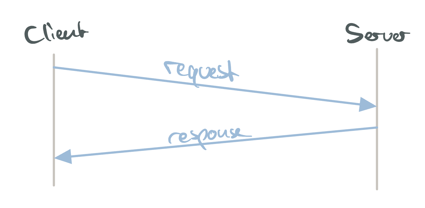
The simplest possible DS, consisting of two nodes sending a message to each other.
There are many possible reasons for choosing to architecting a system in a distributed way:
- The system could, by its very nature, be distributed.
- A DS is typically more reliable.
- A DS might bring better performance (e.g., for geographic reasons).
- A DS can help with data limitations.
- …
In summary, a DS might overcome typical challenges that would otherwise occur with a non-distributed, single-machine system. However, as a tradeoff, any DS will have to overcome new challenges that are not present in a non-distributed system:
- It must be fault-tolerant.
- It must be available.
- It must be able to recover in the case of faults or failures.
- It must be consistent.
- It must be able to scale.
- It must be performant.
- It must be secure.
Concept: System Models
Assuming a bi-directional point-to-point communication between two nodes, the following system model can be derived:
| Part | Option 1 | Option 2 | Option 3 |
|---|---|---|---|
| Network | reliable | fair-loss | arbitrary |
| Nodes | crash-stop | crash-recovery | byzantine |
| Timing | synchronous | partially synchronous | asynchronous |
The options have the following meaning:
- Network:
- reliable: A message is received if, and only if, it is sent.
- fair-loss: Messages may be lost, deduplicated or reordered. If retrying long enough, it will eventually get through.
- arbitrary: A malicious adversary may interfere with messages.
- Nodes:
- crash-stop: A node is faulty if it crashes. Crashed nodes stop forever.
- crash-recovery: A node may crash at any moment, but may resume eventually. Persisted data survives.
- byzantine: A node is faulty if it deviates from the algorithm. Faulty nodes may do anything, including malicious behavior (e.g., dropping all messages).
- Timing:
- synchronous: Message latency has a known upper bound. Nodes execute at a known speed.
- partially synchronous: The system is asynchronous for some finite, unknown time, but synchronous otherwise.
- asynchronous: Messages can be delayed arbitrarily. Nodes can pause arbitrarily. No timing guarantees exist.
The further right the option is in the table, the harder it becomes. Algorithms choose 1 option out of each row that they can handle (e.g., an algorithm could function in a fair-loss network with crash-stop nodes and asynchronous timing).
Concept: Timing and Clocks
Measuring the current time is essential to a DS, e.g., for ordering messages. It is, also, a very hard problem. Time is measured by clocks. We firstly distinguish between these clocks:
- Time-of-day clock: Time since a fixed date.
- Monotonic clock: Time since an arbitrary point in time (e.g., when a machine was started).
In a DS, clocks must be synchronized to adjust/fix a local clock’s drift (deviation). Here, multiple protocols/algorithms exist.
One of them is the Network Time Protocol (NTP) which synchronizes time by sending a request to an NTP server. The server answers with its current time. That + the duration of the request and response allow the client to update its local time.
We can further differentiate between the following clocks:
- Physical clocks: Count the number of seconds elapsed since a given point in time.
- Logical clocks: Count events (e.g., number of messages sent). Designed for capturing causal dependencies. Here, we look at two variants:
- Lamport clock
- Vector clock
The Lamport clock uses the following algorithm. Notably, it maintains an event counter t internally that is incremented whenever an event occurs. The counter is attached to any message sent. Sending/Receiving a message is an event itself and increases the counter. Nodes receiving a message always update their internal counter to the highest known counter.
on initialisation do
  t := 0 // each node has its own local variable t
end on

on any event occurring at the local node do
  t := t + 1
end on

on request to send message m do
  t := t + 1
  send (t, m) via the underlying network link
end on

on receiving (t', m) via the underlying network link do
  t := max(t, t') + 1
  deliver m to the application
end on
A Vector clock, on the other hand, maintains a counter for every node inside a vector (array). The entire vector is delivered with a message:
on initialisation at node i do
  T := (0, 0, ... , 0) // local variable at node N i
end on

on any event occurring at node i do
  T[i] := T[i] + 1
end on

on request to send message m at node i do
  T[i] := T [i] + 1
  send (T, m) via network
end on

on receiving (T', m) at node i via the network do
  T[j] := max(T[j], T'[j]) for every j in {1, ... , n}
  T[i] := T[i] + 1
  deliver m to the application
end on
Vector clocks, in contrast to Lamport clocks, provide information about causality, i.e., which event may have caused another.
Concept: Broadcasts
Broadcasting means delivering a message from one node to all others. Broadcasts build upon System Models. A broadcast can be best-effort (may drop messages), reliable (non-faulty nodes deliver every message, via retries) with either an asynchronous or partially synchronous timing model.
The following reliable broadcasts were presented:
- FIFO broadcast: If one node delivers m1 and m2 and broadcast(m1) happens before broadcast(m2), then m1 must be delivered before m2.
FIFO broadcast can easily be implemented via TCP. - Causal broadcast: If broadcast(m1) happens before broadcast(m2), then m1 must be delivered before m2.
- Total order broadcast: If m1 is delivered before m2 on any node, then m2 must be delivered before m2 on all nodes. There are approaches to a total order broadcast:
- Single leader approach: One node is a leader. Every message goes through the leader.
- Lamport clock approach: Every message has a Lamport clock timestamp attached. A message cannot be delivered before all previous messages have been delivered. Nodes must therefore store newer messages until all previous ones have been received.
- FIFO total order broadcast: FIFO + total order broadcast.
FIFO broadcast algorithm:
on initialisation do
  sendSeq := 0
  delivered := (0, ..., 0)
  buffer := {}
end on

on request to broadcast m at node i do
  deps := delivered
  deps[i] := sendSeq
  send (i, deps, m) via reliable broadcast
  sendSeq := sendSeq + 1
end on

on receiving msg from reliable broadcast at node i do
  buffer := buffer ∪ {msg}

  while ∃(sender, deps, m) 2 buffer.deps <= delivered do
    deliver m to the application
    buffer := buffer \ {(sender, deps, m)}
    delivered[sender] := delivered[sender] + 1
  end while
end on
Causal broadcast algorithm:
on initialisation do
  sendSeq := 0
  delivered := (0, ..., 0)
  buffer := {}
end on

on request to broadcast m at node i do
  deps := delivered
  deps[i] := sendSeq
  send (i, deps, m) via reliable broadcast
  sendSeq := sendSeq + 1
end on

on receiving msg from reliable broadcast at node i do
  buffer := buffer ∪ {msg}

  while ∃(sender, deps, m) ∈ buffer.deps <= delivered do
    deliver m to the application
    buffer := buffer \ {(sender, deps, m)}
    delivered[sender] := delivered[sender] + 1
  end while
end on
Concept: Replication
Replication is the process of keeping multiple copies of data on multiple machines. Replicas are, due to the distributed nature, frequently out of sync and must reconcile (i.e., synchronize their states). This can become troublesome when clients read/write concurrently on different out-of-sync replicas, e.g., because two clients might read different values.
Concurrent writes can be solved via two approaches: Last writer wins or Multi-value register (timestamps with partial order, where two concurrent values can both be kept).
Read after write concurrency (i.e., after writing to one replica, reading the same value from a different replica) can be solved via quorums.
State Machine Replication (SMR) is an approach to make replicas fault tolerance. It builds upon the fact that state machines are deterministic: For a given input, a state machine will always produce a given output. Applied to a DS, it is possible to make each replica a state machine. By observing the output of each other, replicas notice when another replica becomes faulty (this is the case when the output of a replica deviates from the expected output).
SMR uses FIFO total order broadcast for every update on all replicas. Applying an update is deterministic.
on request to perform update u do
  send u via FIFO-total order broadcast
end on

on delivering u through FIFO-total order broadcast do
  update state using arbitrary deterministic logic
end on
Concept: Linearizability
Linearizability is a strong correctness/strong consistency condition, where a set of concurrent operations on multiple machines can be reordered/executed in a way, as if they were running on a single machine. Every operation takes effect atomically sometime after started and ended.
Linearizability is not present by default, but can, in many cases, be achieved via specific approaches or algorithms. An example is the ABD algorithm:
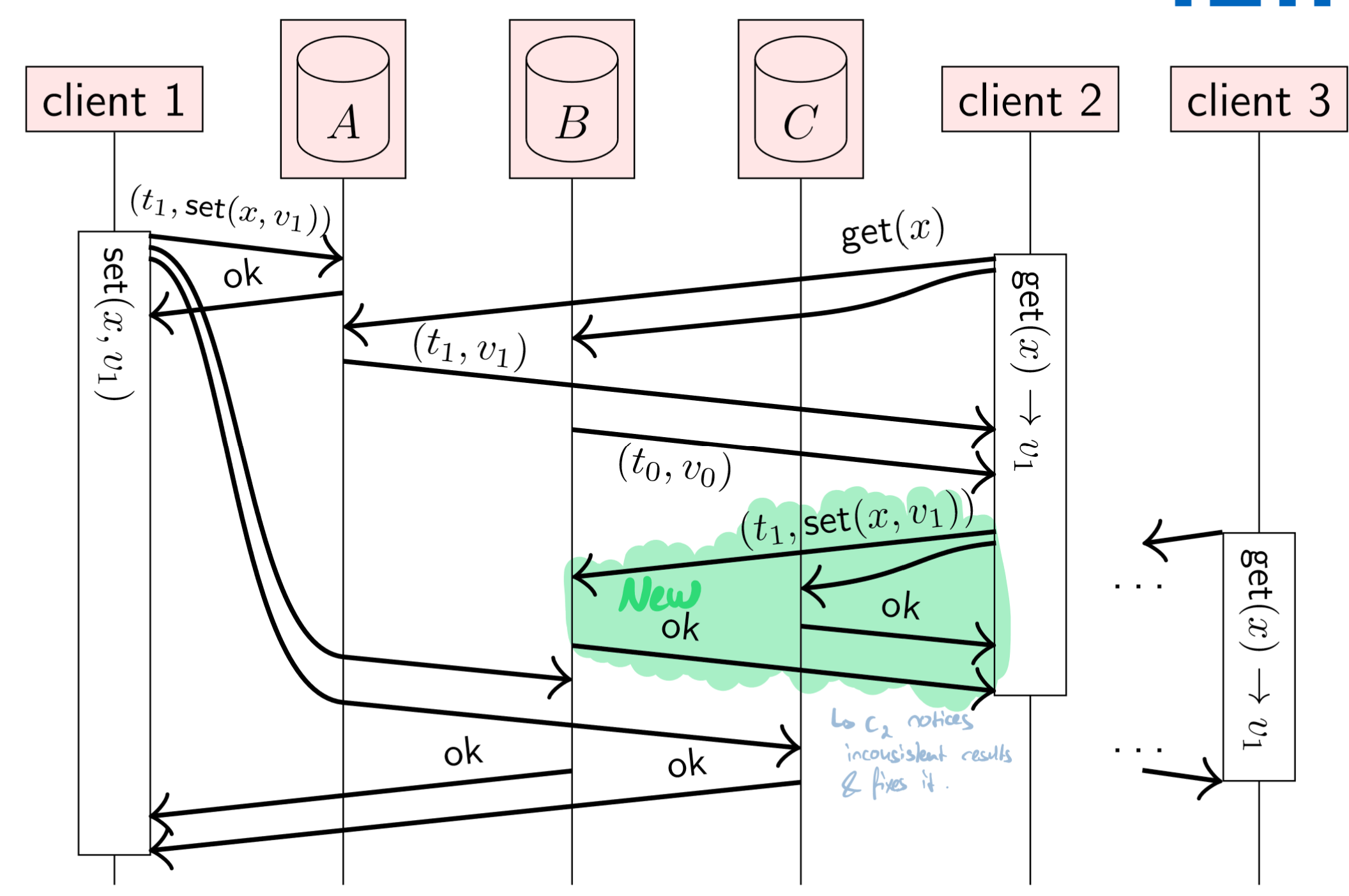
ABD algorithm. (Source: Lecture Slides)
The part highlighted in green ensures linearizability. Without it, client 3 would not read the value written by client 1, despite a quorum (because the replicas from which client 3 reads haven’t received notice of the change yet).
It’s even possible to write a linearized compare-and-swap (CAS) operation in a DS:
on request to perform get(x) do
  total order broadcast (get, x) and wait for delivery
end on

on request to perform CAS(x, old, new) do
  total order broadcast (CAS, x, old, new) and wait for delivery
end on

on delivering (get, x) by total order broadcast do
  return localState[x] as result of operation get(x)
end on

on delivering (CAS, x, old, new) by total order broadcast do
  success := false

  if localState[x] = old then
    localState[x] := new
    success := true
  end if

  return success as result of operation CAS(x, old, new)
end on
Concept: Consensus
Motivation: For a fault-tolerant total order broadcast using a leader, it’s required to be able to automatically elect a new leader. This requires consensus among the nodes.
Consensus generally means having multiple nodes agree on a single value. This can be used for leader election.
One algorithm for leader election is Raft. Raft elects one leader per term. A new term is started when the old leader becomes faulty. Raft can only guarantee one leader per term, but must allow multiple leaders from different terms at a given point in time. In Raft, nodes may take on the following states:
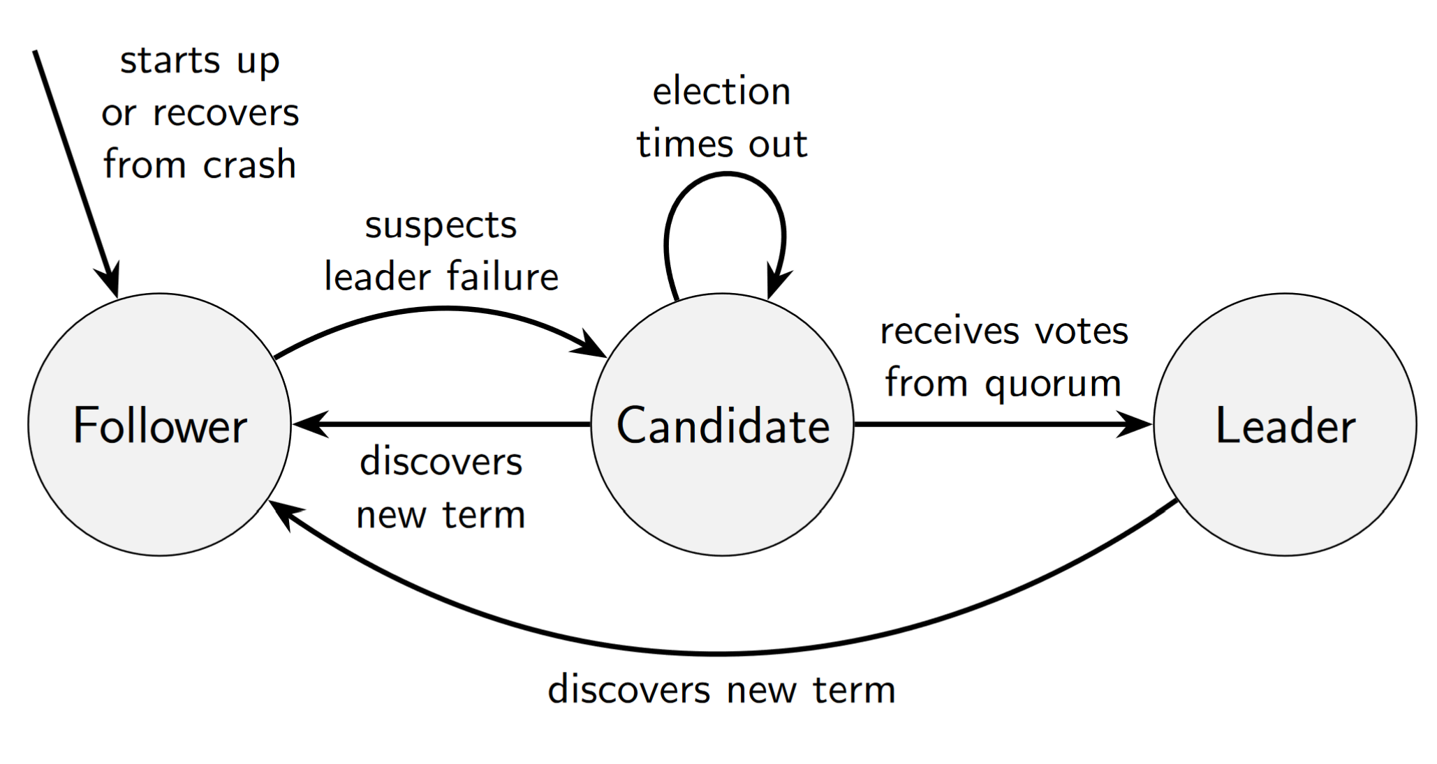
Raft node state transitions. (Source: Lecture Slides)
on initialisation do
  currentTerm := 0
  votedFor := null
  log := ()
  commitLength := 0
  currentRole := follower
  currentLeader := null
  votesReceived := {}
  sentLength := ()
  ackedLength := ()
end on

on recovery from crash do
  currentRole := follower
  currentLeader := null
  votesReceived := {}
  sentLength := ()
  ackedLength := ()
end on

on node nodeId suspects leader has failed, or on election timeout do
  currentTerm := currentTerm + 1
  currentRole := candidate
  votedFor := nodeId
  votesReceived := {nodeId }
  lastTerm := 0

  if log.length > 0 then
    lastTerm := log[log.length - 1].term
  end if

  msg := (VoteRequest, nodeId, currentTerm, log.length, lastTerm)

  for each node of nodes
    send msg to node
  end for each

  start election timer
end on

on receiving (VoteRequest, cId, cTerm, cLogLength, cLogTerm) at node nodeId do
  if cTerm > currentTerm then
    currentTerm := cTerm
    currentRole := follower
    votedFor := null
  end if

  lastTerm := 0

  if log.length > 0 then
    lastTerm := log[log.length - 1].term
  endif

  logOk := (cLogTerm > lastTerm) ||
    (cLogTerm = lastTerm && cLogLength >= log.length)

  if cTerm = currentTerm && logOk && votedFor in {cId null} then
    votedFor := cId
    send (VoteResponse, nodeId, currentTerm, true) to node cId
  else
    send (VoteResponse, nodeId, currentTerm, false) to node cId
  end if
end on

on receiving (VoteResponse, voterId, term, granted) at nodeId do
  if currentRole = candidate && term = currentTerm && granted then
    votesReceived := votesReceived union {voterId}

    // Quorum reached?
    if |votesReceived| >= ceil((|nodes| + 1) / 2) then
      currentRole := leader
      currentLeader := nodeId
      cancel election timer

      for each follower in nodes \ {nodeId} do
        sentLength[follower] := log.length
        ackedLength[follower] := 0
        ReplicateLog(nodeId, follower)
      end for each
    end if
  else if term > currentTerm then
    currentTerm := term
    currentRole := follower
    votedFor := null
    cancel election timer
  end if
end on

on request to broadcst msg at node nodeId do
  if currentRole = leader then
    append the record (msg : msg, term : currentTerm) to log
    ackedLength[nodeId] := log.length

    for each follower in nodes \ {nodeId} do
      ReplicateLog(nodeId, follower)
    end for each
  else
    forward the request to currentLeader via FIFO link
  end if
end on

periodically at node nodeId do
  if currentRole = leader then
    for each follower in nodes \ {nodeId} do
      ReplicateLog(nodeId, follower)
    end for each
  end if
end do

// Only called on leader whenever there is a new message in the log + periodically.
function ReplicateLog(leaderId, followerId)
  prefixLen := sentLength[followerId]
  suffix := (log[prefixLen], log[prefixLen + 1], ..., log[log.length - 1])
  prefixTerm := 0

  if prefixLen > 0 then
    prefixTerm := log[prefixLen - 1].term
  end if

  send (LogRequest, leaderId, currentTerm, prefixLen, prefixTerm, commitLength, suffix) to followerId
end function

// follower receiving messages
on receiving (LogRequest, leaderId, term, prefixLen, prefixTerm, leaderCommit, suffix) at node nodeId do
  if term > currentTerm then
    currentTerm := term
    voedFor := null
    cancel election timer
  end if

  if term = currentTerm then
    currentRole := follower
    currentLeader := leaderId
  end if

  logOk := (log.length >= prefixLen) && (prefixLen = 0 || log[prefixLen - 1].term = prefixTerm)

  if (term = currentTerm && logOk then
    AppendEntries(prefixLen, leaderCommit, suffix)
    ack := prefixLen + suffix.length
    send (LogResponse, nodeId, currentTerm, ack, true) to leaderId
  else
    send (LogResponse, nodeId, currentTerm, 0, false) to leaderId
  end if
end on

// update followers' logs
function AppendEntries(prefixLen, leaderCommit, suffix)
  if suffix.length > 0 && log.length > prefixLen then
    index := min min(log.length, prefixLen + suffix.length) - 1

    if log[index].term != suffix[index - prefixLen].term then
      log := (log[0], log[1], ..., log[prefixLen - 1])
    end if
  end if

  if prefixLen + suffix.length > log.length then
    for i := log.length - prefixLen to suffix.length - 1 do
      append suffix[k] to log
    end for
  end if

  if leaderCommit > commitLength then
    for i := commitLength to leaderCommit - 1 do
      deliver log[i].msg to the application
    end for

    commitLength := leaderCommit
  end if
end function

// leader receiving acks
on receiving (LogResponse, follower, term, ack, success) at nodeId do
  if term = currentTerm && currentRole = leader then
    if success && ack >= ackedLength[follower] then
      sentLength[follower] := ack
      ackedLength[follower] := ack
      CommitLogEntries()
    else if sentLength[follower] > 0 then
      sentLength[follower] := sentLength[follower] - 1
      ReplicateLog(nodeId, follower)
    end if
  else if term > currentTerm then
    currentTerm := term
    currentRole := follower
    votedFor := null
    cancel election timer
  end if
end on

// leader committing log entries
define acks(length) = |{n in nodes | ackedLength[n] >= length}|

function CommitLogEntries()
  minAcks := ceil((|nodes| + 1) / 2)
  ready := {len in {1, ..., log.length} | acks(len) >= minAcks}

  if ready != {} && max(ready) > commitLength && log[max(ready) - 1].term = currentTerm then
    for i := commitLength to max(ready) - 1 do
      deliver log[i].msg to the application
    end for

    commitLength := max(ready)
  end if
end function
Concept: Eventual Consistency
While Linearizability is a strong model, it has disadvantages in the form of performance, scalability and availability. Sometimes, weaker models are enough for a DS. One such model is eventual consistency. It states that if there are no more updates, then all replicas will eventually be in the same state.
Strong eventual consistency improves on the “no more updates” part via the following points:
- Eventual delivery: Every update made to one non-faulty replica is eventually processed by every non-faulty replica.
- Convergence: Any replicas which have processed the same updates are in the same state.
Concept: RPC (Remote Procedure Call)
RPC is a concept that leverages a DS to execute a function (or procedure) on a remote machine. This is hidden from the caller of the function (location transparency).
A prominent example is a transaction of money:
// At the client:
let result = processPayment({
  card: '123456',
  amount: 13.0,
});

log('Result: ' + result.ok);
In the above example, the processPayment function is not executed locally on the client, but instead on another node. Both the function’s argument and the result are (un-)marshalled before/after being sent/received over the network.
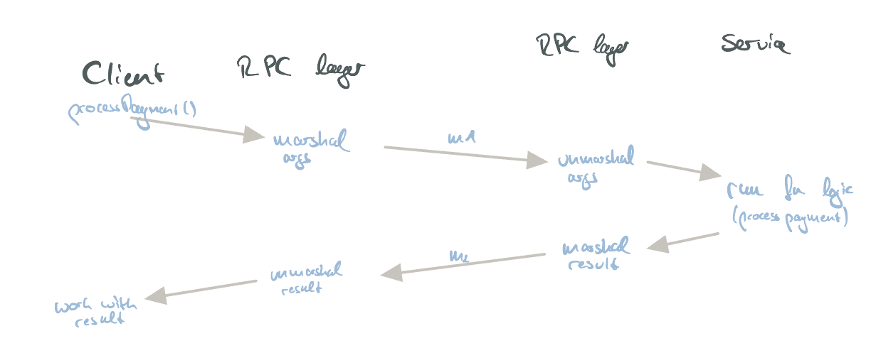
The internals of the RPC request/response flow.
RPCs are very common in todays applications. Examples of prominent RPC frameworks/technologies are:
- gRPC
- REST
- Java RMI
Concept: Leases
📄 Papers: 1
Leases address the general issue of acquiring exclusive read- or write-access to a resource. They solve a problem of traditional locks applied to a DS: That any node which acquired a lock can crash or have a network failure, resulting in the lock never being released.
Leases address this underlying problem by applying a timeout. A client can request a lease (“lock”) for a resource for a limited amount of time and, if required, renew that lease. Once the lease expires, the resource is usable by other nodes again.
There are, typically, two types of leases:
- Read leases (allows many concurrent readers).
- Write leases (allows one single writer).
Servers may further forcibly evict clients holding a lease if required.
Concept: Key-Value (KV) Stores
KV stores are NoSQL-like, distributed systems which are able to store massive amounts of values indexed by a key. At their core, they have a very slim API surface:
get(key);
put(key, value);
delete key;
This simple API brings a lot of benefits in a distributed world: Reliability, high availability, high performance, horizontal scalability, etc. The tradeoff being made is the lack of a data schema (which becomes apparent when comparing a KV store with a fully-fledged SQL database).
Prominent examples of KV stores are:
- BigTable
- Apache HBase
- Apache Cassandra
- Redis
- Amazon Dynamo
KV stores typically build upon a concept called consistent hashing.
KV stores typically replicate values. KV pairs can be read from any replica.
For a real-life example, see Cassandra.
Concept: Consistent Hashing
Consistent hashing addresses the problem of mapping objects to caches. Given a number of caches, each cache should hold an equal share of cachable objects. Clients need to know which cache to contact to avoid cache misses. The key issue to be solved here is how to partition the objects in a non-skewed distribution, i.e., in a way where object identifiers are evenly mapped to the available caches. Given a uniformly distributed hash function, hashing is one way to solve this.
The problem with using “normal hashing” is that, on failure of a cache node, other nodes would have to repopulate their internal cache. This would cause a lot of inefficient cache misses:
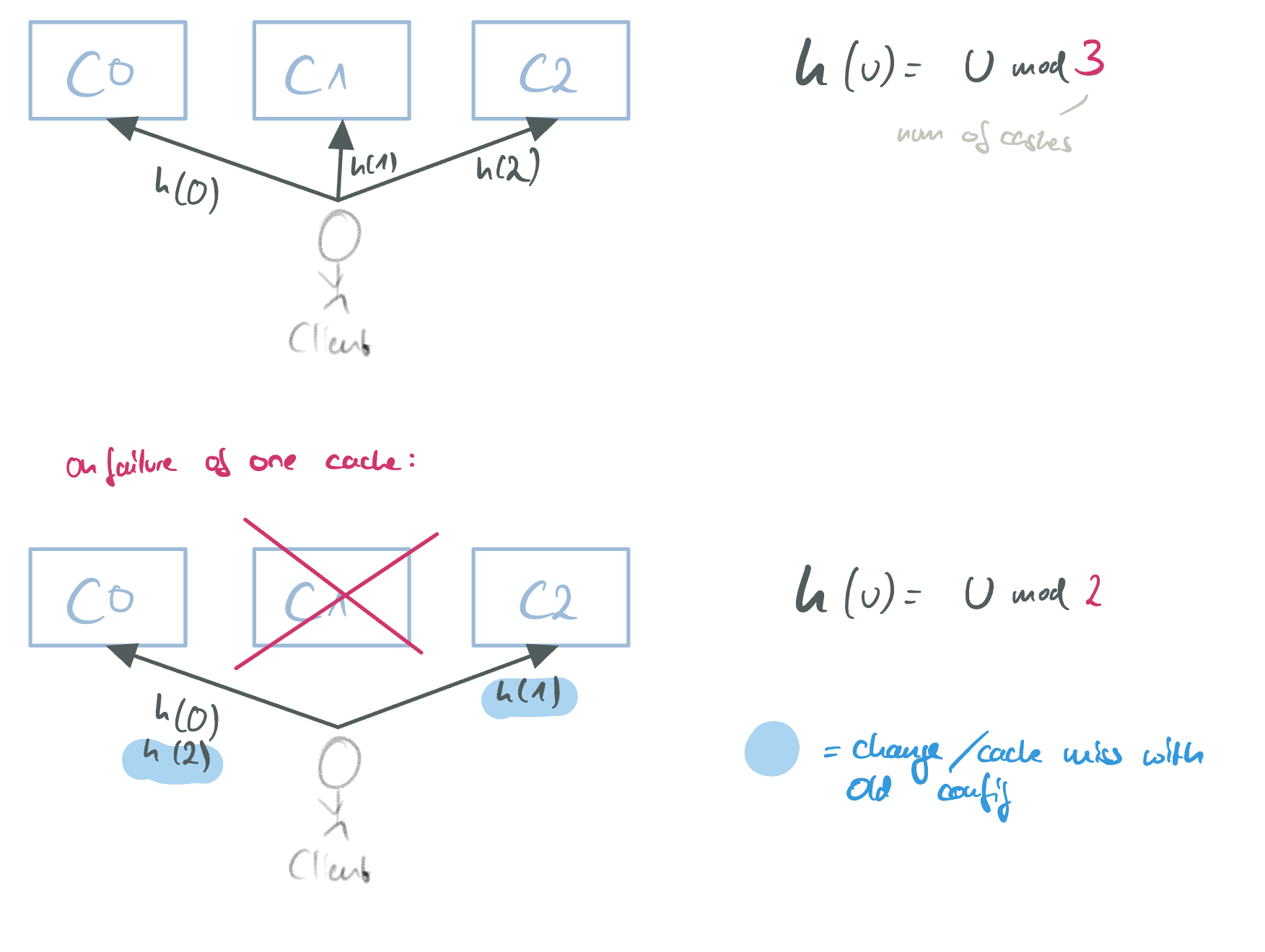
The problem of not using consistent hashing.
Consistent hashing solves the issue by allowing the addition/removal of cache nodes without (much) disruption. Consistent hashing is implemented via a key ring and a hash function that uniformly distributes the results over an interval [0, M] where M indicates the number of cache nodes. Each cache node is placed at a certain position of the key ring. A node is responsible for every key <= its position. When new nodes are added, they take over the responsibility for their new key ring section from the node that previously handled them. When nodes fail, the successor node takes over the failed nodes responsibilities. Node addition/removal can be coordinated via gossiping or a central coordinator service. The following image shows an example:
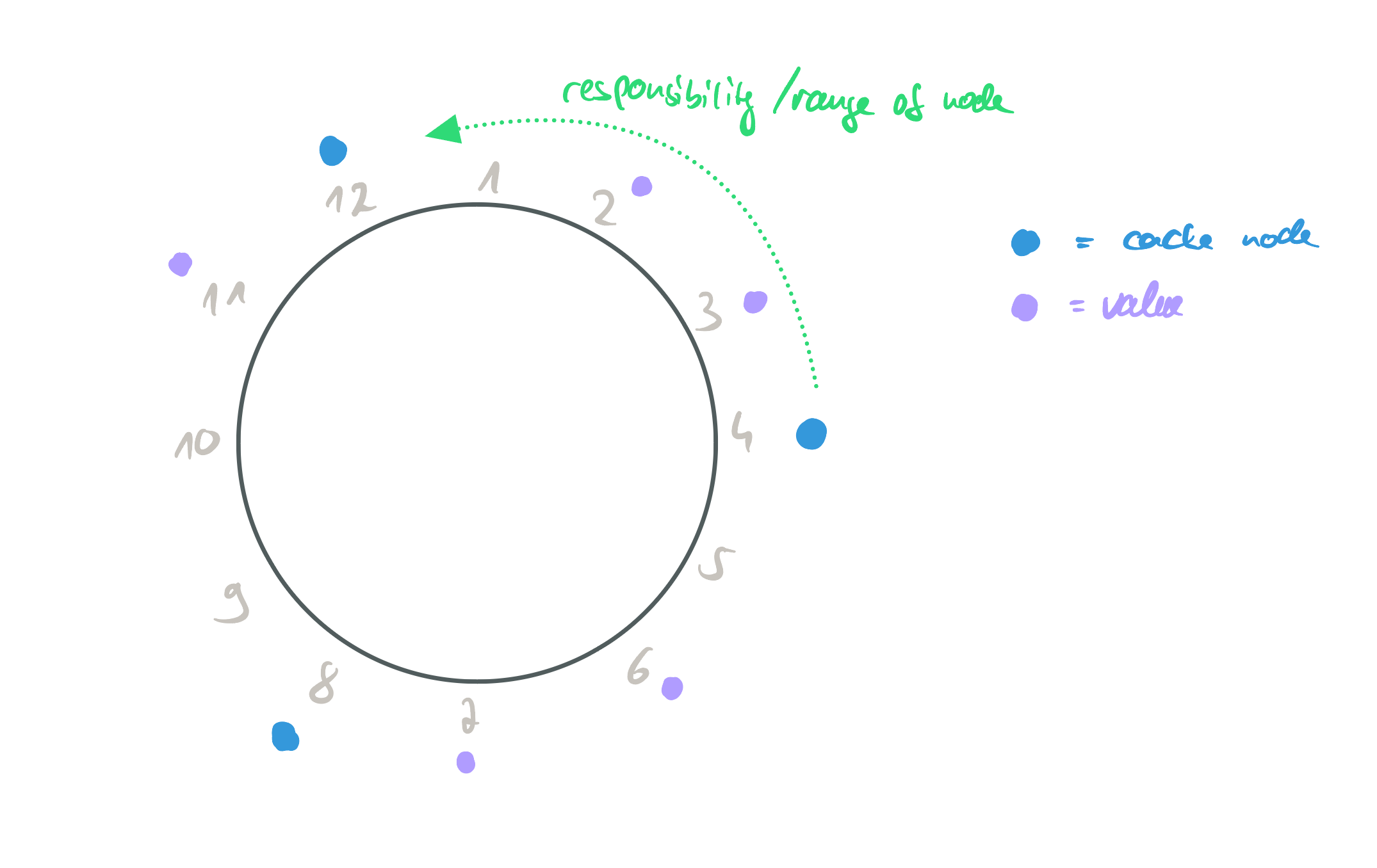
Consistent hashing applied.
When a client wants to do a lookup, he needs to fetch the information about which cache node is responsible for the (hashed) key. He can then (depending on the system, of course) directly contact that node. The cache lookup data structure can be implemented as a binary tree for O(log n) lookups (but other solutions exist as well).
Concept: Log Structured Merge-Trees (LSM)
LSMs are a data structure which became popular for NoSQL systems. It combines the benefits of RAM and hard drives (i.e., fast access and persistence). They provide a very simple API:
get(key);
put(key, value);
LSMs leverage three key data structures:
- MemTable: A KV data structure kept entirely in-memory. Uses a Skip list for fast value access.
- SSTable: A persistent, disk-based data structure. Stores immutable KV pairs.
- WAL: Append-only log file for fault tolerance (supports UNDO And REDO logs).
In practice, these data structures work together like this:
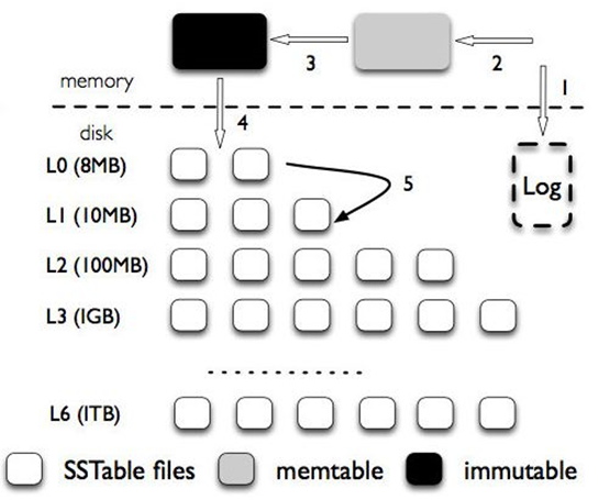
LSM Architecture. Source
- New KV pairs are immediately added to the WAL (allows recovery).
- KV pair is added to MemTable.
- Once MemTable runs out of space: It is made immutable. A new MemTable is created.
- Immutable MemTables can be stored on disk. Here, multiple layers exist, continuously increasing in size. Newer entries are stored in the upper layers. Lookups go through the layers, in order.
LSMs use a compaction phase (i.e., “garbage collection”) in the background to merge SSTables from different layers (older keys are updated with newer values - the old values are discarded).
LSMs don’t support “traditional” deletes. Instead, deleted KV pairs are marked with a tombstone (and can be removed in the upcoming compaction phases).
Case Study: MapReduce
📄 Papers: 1
MapReduce is a model/library introduced by Google. It provides an abstraction for processing large amounts of data on multiple distributed machines. It provides a slim API to application developers, inspired by FP concepts:
map(key, value): (key, value)reduce(key, value): (key, value)
Application developers only need to implement these two functions when using MapReduce. MapReduce itself then handles the entire complexity of that come with distributed data processing: parallelization, communication, load balancing, fault tolerance, synchronization, scheduling, …
Internally, MapReduce processes data in three phases: Map, Shuffle and Reduce:
- Map: User-provided. Maps a KV pair to another KV pair. Essentially transforms the data.
- Shuffle: Handled by MapReduce. Groups all results of the Map phase by the resulting keys.
- Reduce: User-provided. Aggregates/Reduces the values of a single key (i.e., a group returned by the Shuffle phase) into one final result.
A simple demo use-case is counting the amount of words in documents. Here, we can define the following Map/Reduce functions, resulting in the following MapReduce flow:
map(key: string, value: string) {
  foreach (word of value.split(" "))
    yield return (word, 1);
}

reduce(key: string, value: Iterator<string>) {
  return (key, value.cast<Int>().sum().cast<string>());
}
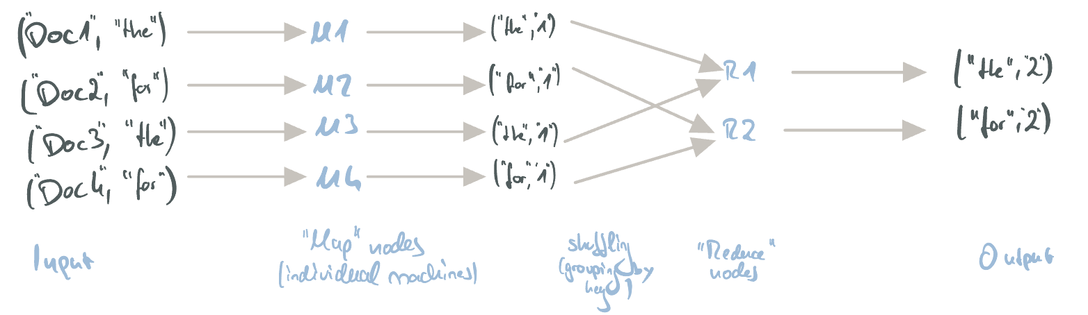
The MapReduce flow for counting words in documents.
Internally, MapReduce uses a master/slave architecture and a distributed file system (GFS/HDFS). The master node takes care of job tracking (i.e., task assignment) while the slave nodes are the workers executing the Map/Reduce tasks.
Case Study: (Apache) Pig
MapReduce is powerful, but is a lower-level abstraction that, while handling the complexity of a DS, leaves a lot of work remaining for the application developer. Many common tasks, especially in the area of data analysis (filter, join, group, …) is missing in MapReduce.
Pig is a framework which builds upon MapReduce and provides these operations via the Pig Latin language. Pig Latin is an SQL-like, imperative language that is compiled into several MapReduce steps. This compilation process enables optimizations and simplifications in otherwise complex and potentially slow MapReduce applications.
The Pig compiler uses the following transformation structure: Logical plan ➡️ Physical plan ➡️ MapReduce plan. The last plan, MapReduce, is a sequence of multiple MapReduce programs that represent the initial Pig program. The following image shows the tiered compilation process:
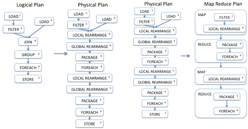
Pig’s plan transformation. Source
Case Study: Google File System (GFS) / Hadoop Distributed File System (HDFS)
📄 Papers: 1
Distributed file systems provide a FS spread out over various machines. Users of the FS do not necessarily notice this and may interact with the FS as if it was provided by the local device. Making a file system distributed massively increases the amount of storeable data and bandwidth, while, as a tradeoff, bringing all of the complexities of a DS.
A distributed FS is often the very bottom layer of a DS, because reading/writing files is typically a core requirement of any application. As such, it is, for example, typical to see MapReduce applications written on top of a distributed FS.
GFS/HDFS are distributed FS implementations. GFS specifically was invented by Google to address internal requirements like large files, large streaming reads, concurrent appends, high bandwidth, etc. HDFS was introduced in the lecture as the open-source variant of GFS. In the following, details of GFS are described.
GFS: Architecture Overview
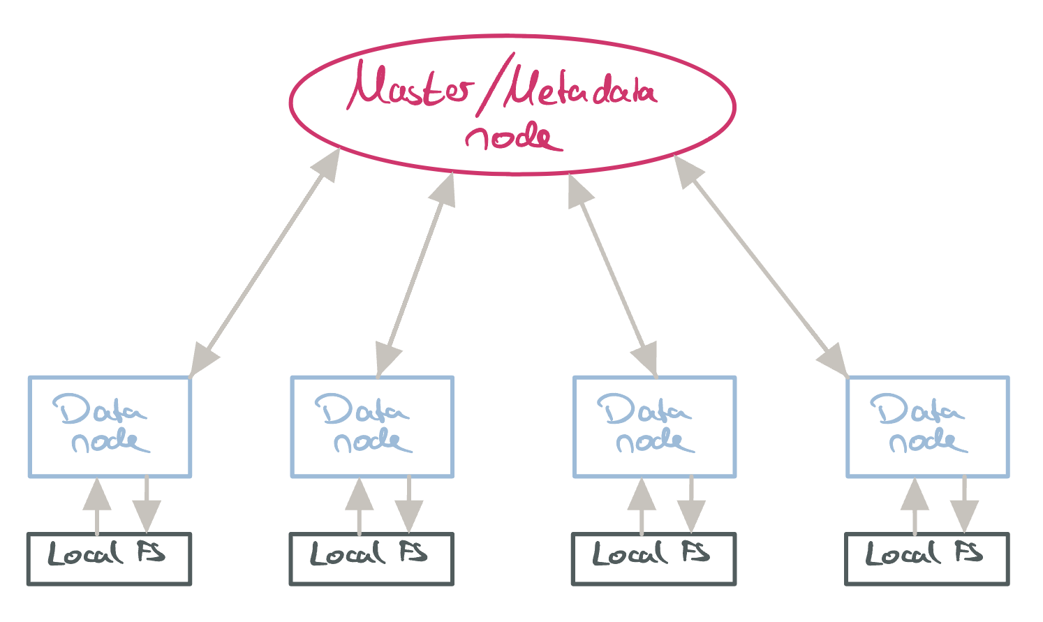
GFS Architecture.
GFS typically has a master/coordinator node which provides metadata information to clients about data nodes. Data nodes (also called chunk servers) are responsible for storing the actual FS data. Here, they use the machine’s local FS for storage. The master node is made aware of the available data nodes via heartbeats. Due to the master node being centralized, clients will try to minimize the time spent interacting with it. Generally, clients will talk to data nodes directly. They do have to contact the master node for getting the data node metadata though (and for acquiring a lease on that node):
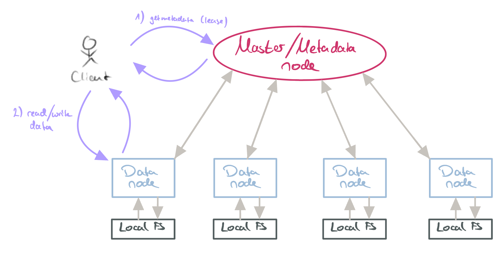
GFS data access.
GFS structures files into various chunks (with a length of 64MB). These chunks are replicated accross multiple data nodes. When clients want to read/write a chunk, they talk to the master node which provides the chunk location. Clients are then free to choose any replica holding the chunk (and will typically choose the closest).
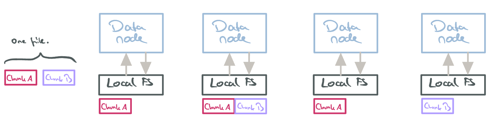
Chunks in GFS. Note that the file is spread over different data nodes/replicas.
GFS: Reading and Writing Data
Reading data is straightforward: The client contacts the data node containing the chunk of interest. Writing data is, however, more complex. The following image shows the required steps. Briefly, the following happens:
- The client retrieves the data node locations from the master.
- The client pushes the data to all replicas.
Note that the client only makes one request: The replicas forward the request to the nearest, next replica. - The client asks the primary replica to finalize the write. The primary forwards this request to the secondary replicas.
- If everything succeeded, the client is notified. If not, he will retry.
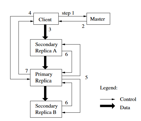
Writing data in GFS. Source
Writes in GFS are consistent, but undefined. This is the case because it’s possible for file regions to end up containing mingled fragments from different clients. “Consistent”, in this case, means that all clients will see the same results. This result may not be what the client wrote. In contrast, a chunk/region is called “defined”, if the result is exactly what the client wrote. See the following table for overall consistency guarantees:
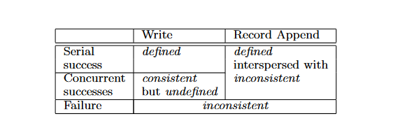
GFS Consistency Guarantees. Source
Case Study: Zookeeper
📄Papers: 1
Zookeeper is a microkernel-like application which, as a kernel, provides a foundation for other distributed systems. It provides a slim API surface which can be used for common tasks/challenges like configuration, naming, synchronization, discovery, group services, … Internally, Zookeeper uses a cluster of servers with one leader to serve an arbitrary number of clients.
Zookeeper uses/guarantees FIFO-ordering for clients, Linearizable writes and a wait-free API.
Each Zookeeper server keeps a full copy of the state in-memory.
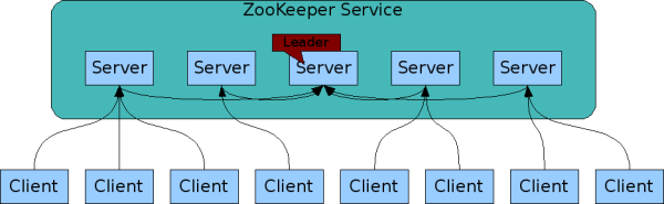
Zookeeper Architecture. Source
Zookeeper stores data in a hierarchy. The nodes are called znodes. These can store arbitrary data. A znode can be regular (persistent, client-managed) or ephemeral (deleted once the session of the creator client expires). A znode can also be flagged as sequential (resulting in increasing counters) and/or as watched (clients will be notified about changes). These foundations result in the following API:
create(path, data, flags);
delete (path, version); // Version is used for conditional updates.
exists(path, watch);
getData(path, watch);
setData(path, data, version); // Version is used for conditional updates.
getChildren(path, watch);
sync(); // To flush() changes.
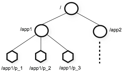
A Zookeeper znode hierarchy. Source
Zookeeper: Practical Examples
Configuration: Get/Set shared settings.
// Get config and be notified about changes:
let currentConfig = getData('.../config/settings', true)

// Update config:
setData('.../config/settings', newConfig)

// Update local config value on change:
onConfigChanged() {
  getData('.../config/settings', true)
}
Group Membership: Register clients as znodes which persist while the client is alive. Get all currently active clients as a leader.
// Register myself in the "worker" group:
create('.../workers/myClient', myClientInfo, EPHEMERAL);

// Leader: get group members (and be notified about changes):
let members = getChildren('.../workers', true);
Leader Election: Find the leader or try to become the leader if no leader exists.
let leader;
while (!leader) {
  leader = getData('.../workers/leader', true) || create('.../workers/leader', myClientInfo, EPHEMERAL);
}
Mutex: Create a single mutex.
if (create('.../mutex', EPHEMERAL)) {
  // Mutex acquired!
} else {
  // Wait for release:
  getData('.../mutex', true);
}
Zookeeper Atomic Broadcast (ZAB)
📄 Papers: 1
ZAB is a crash-recovery atomic broadcast algorithm used internally by Zookeeper. It guarantees at-least-once semantics (state changes are idempotent). Zookeeper assumes fair-lossy links and uses TCP to ensure FIFO order. Internally, Zookeeper uses a primary-backup scheme to maintain a consistent replica state. Here, a single primary process receives all client requests and forwards them, in order, to replicas via ZAB. The flow is depicted in the following image:
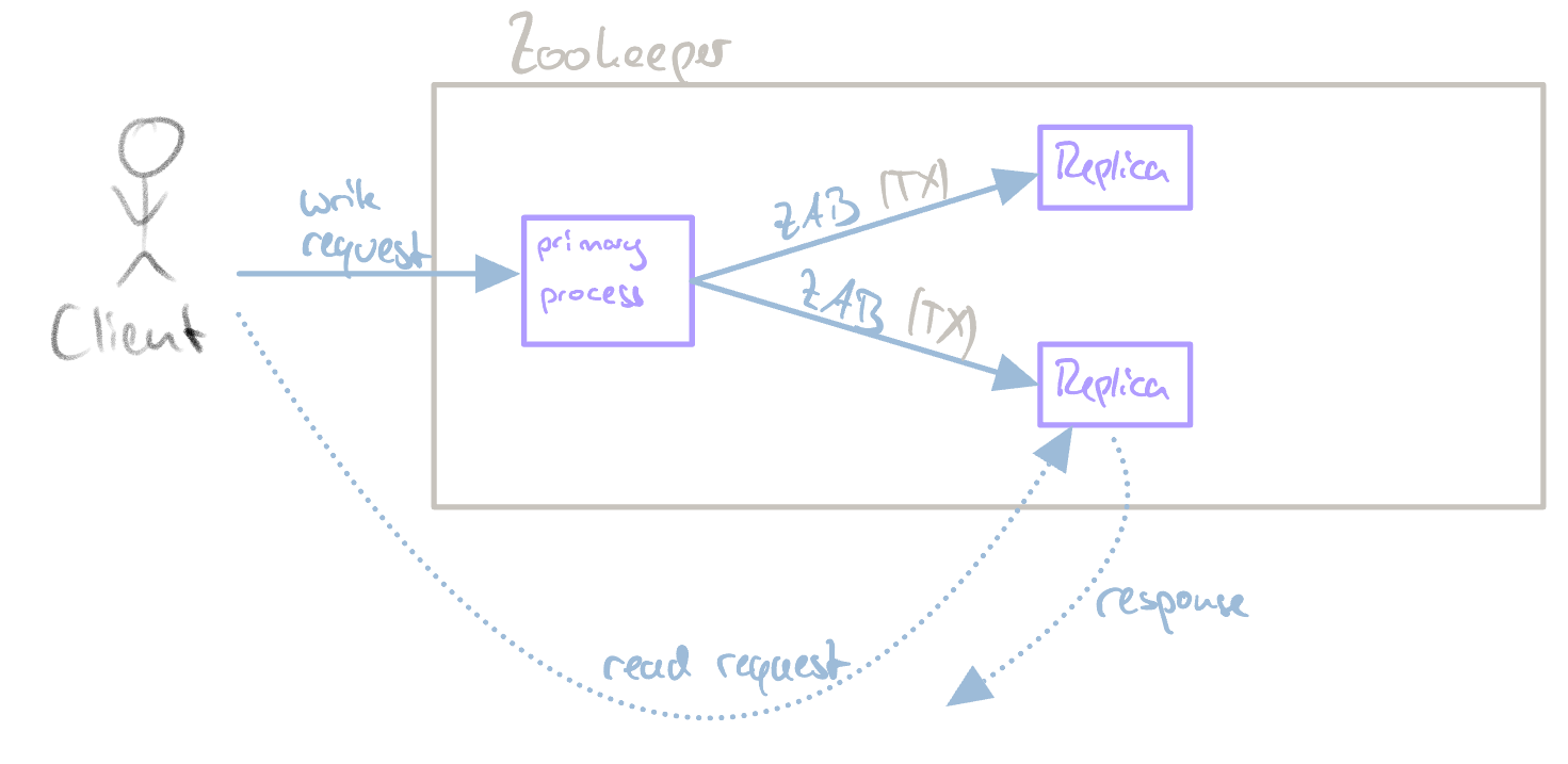
ZAB flow for read/write requests.
ZAB is used for crash recovery. When a primary crashes, other process first agree upon a common state and then elect a new primary via a quorum. There can only ever be one active primary.
State changes are called transactions (TX). Each TX is identified by a tuple (zxid, value) , where zxid is another tuple (epoch, counter), where epoch is a counter that increases whenever the primary changes and counter is a number that increases with each new transaction. Therefore, zxid tuples can be ordered (first by the epoch, then by the counter).
Zookeeper requires the following safety properties to work properly:
- Integrity: In order to deliver a message, a process must have received that very same message.
- Total order/Primary order: If a message a is delivered before message b by a process, all other process must also deliver a before b.
- Agreement: Any two processes deliver the same message.
- Primary integrity: A primary broadcasts only once it has delivered the TXs of previous epochs (for recovery).
As mentioned before, a process in ZAB can be assigned two roles: leader and follower. To determine the current leader, ZAB uses three phases: discovery, synchronization and broadcast. Each process, independent of its current phase, has an internal leader oracle telling which process is currently supposed to be the leader (a process can reference itself here). Note that this information may not be accurate - to become a leader, all three phases have to be run through. Zookeeper discovers failures via heartbeats. On failure, the discovery phase is started with a leader election. The full ZAB algorithm plays out like this:
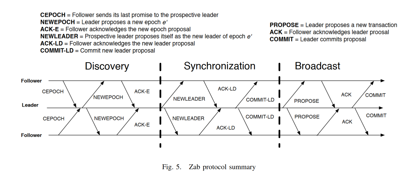
The ZAB protocol, running through the three ZAB phases. Source
The above image shows the entire algorithm. The three phases can be explained in a more simplified manner like this:
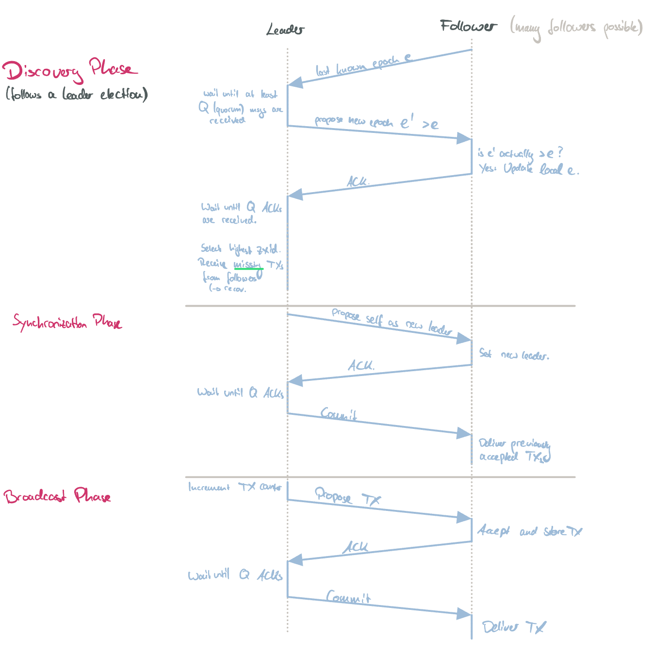
The ZAB protocol, running through the three ZAB phases (simplified).
Case Study: Cassandra
Cassandra is an eventually consistent KV Store developed by Facebook. It’s based on Amazon Dynamo (a closed-source variant). Cassandra uses a decentralized architecture (i.e., no master assignment) and consistent hashing. Information is exchanged via gossiping.
Internally, Cassandra is architected and processes reads/writes like this:
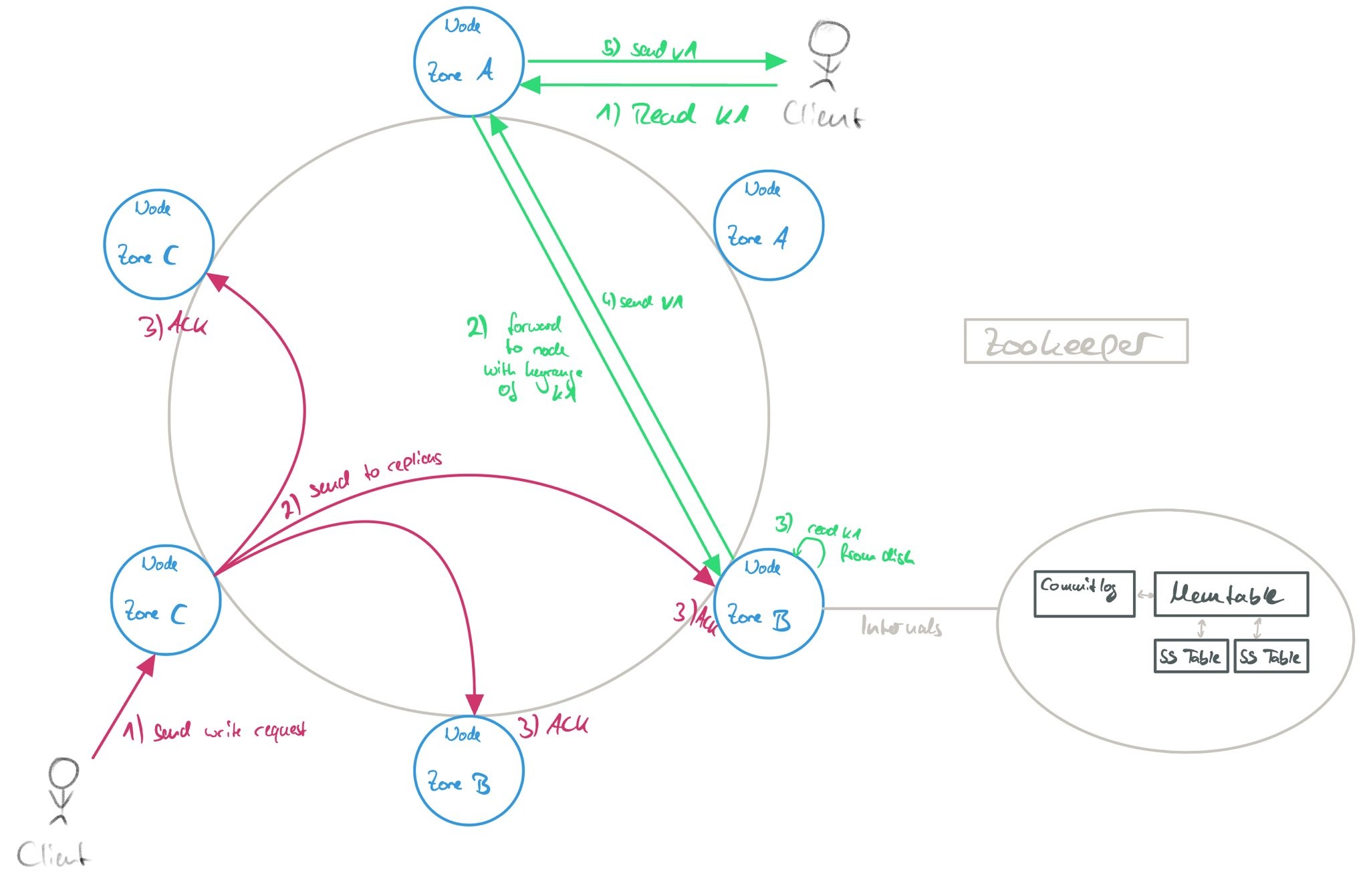
Cassandra internals and read/write behavior.
Case Study: Google’s BigTable
📄 Papers: 1
BigTable is a distributed DB for storing structured data. It focuses on being scalable, efficient, and self-managing. Google introduced it to solve their high data demands.
One “BigTable” is a sparse, distributed, persistent multi-dimensional sorted map. Values can be accessed via the following lookup function: lookup(key: (row, column, time)): value.
BigTable organizes data via rows, columns + column families (e.g., for access control) and multiple values versioned by UNIX timestamps.
For distributing and load-balancing, a range of rows is organized into a tablet.
In summary, a BigTable is structured like this:
| Column Family 1 | Column Family 2 | ||||
|---|---|---|---|---|---|
| Row | Col 1 | Col 2 | Col 3 | Col 1 | Col 2 |
| 1 | V1 @ T1 | V2 @ T1 | V3 @ T1 | V4 @ T1 | V5 @ T1 |
| V1 @ T2 | |||||
| 2 | … |
BigTable offers the following (sketched out) API:
// Table management:
createTable()
deleteTable()
...

// CRUD:
createRow()
readRow()
updateRowAtomic()
updateRowConditionally()
deleteRow()
singleRowTx()

// Scan:
rowIterator()
BigTable uses the following architecture:
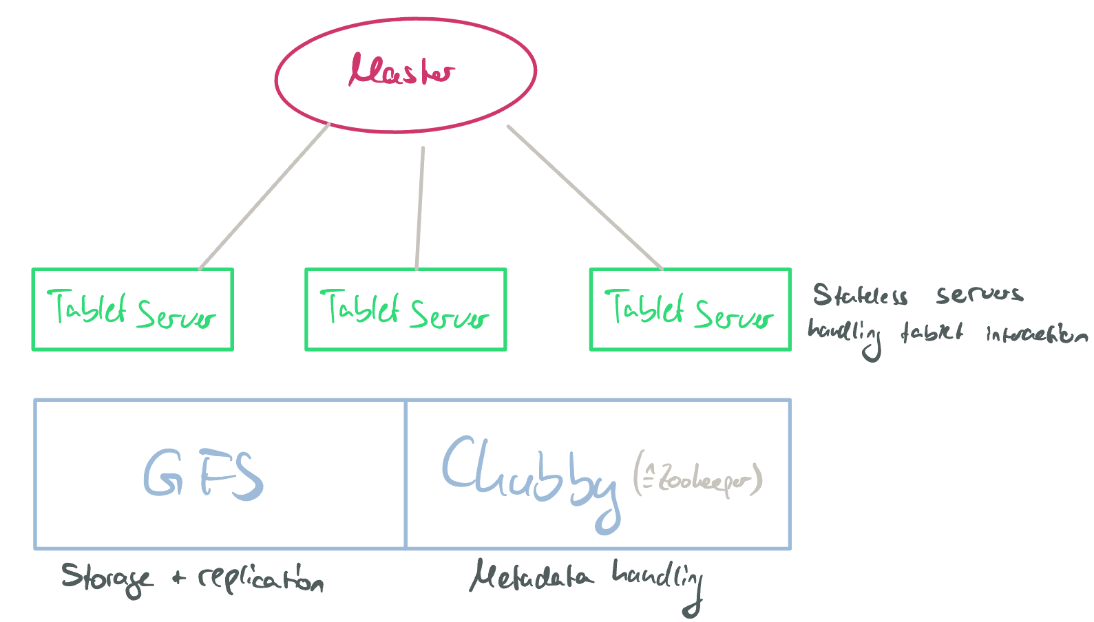
BigTable architecture.
Here, the nodes have the following responsibilities:
- Master:
- Assigns tablets to tablet servers.
- Detects faulty servers.
- Handles garbage collection of deleted tablets.
- Coordination (metadata, schema updates, …).
- DOES NOT provide locations of tablets.
- Tablet server:
- Handles R/W requests of clients.
- Splits large tablets.
- Manages tablets on GFS.
- Caches frequently accessed data.
- DOES NOT hold any state - this is done entirely by GFS (which then also takes care of fault tolerance).
- Chubby:
- Stores system metadata.
- Handles tablet location.
Case Study: Google’s Spanner
📄 Papers: 1
Spanner is a globally-distributed, scalable, multi-version DB developed by Google. A key point of interest is that it supports externally-consistent, linearizable, distributed transactions. Distributed transactions with strong semantics are, fundamentally, a very hard problem to solve.
Spanner thus “competes” with BigTable, though they solve different goals: BigTable has weak semantics (specifically, no transaction support beyond one row), while Spanner provides strong semantics (distributed multi-row transactions).
Spanner builds upon the following techniques to achieve its goal:
- State Machine Replication within a shard (via Paxos)
- 2PL for serialization
- 2PC for distributed transactions
- Multi-version DB systems
- Snapshot isolation
Spanner introduced a novel concept: Global wall-clock time / TrueTime. Previous systems assumed that a global time was not possible. Spanner introduces such a global time that is respected by every timestamp inside the system (resulting in timestampOrder == commitOrder). The TrueTime API exposes time as an interval [earliest, latest] and not as a fixed timestamp. The interval is based on an error term ε, where latest - earliest == ε, i.e., interval.length == ε. ε is calculated based on time values provided by different servers.
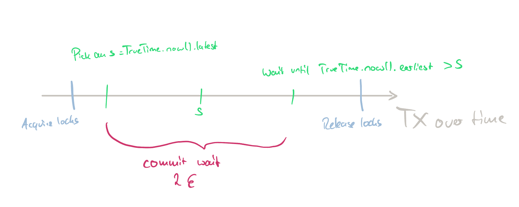
TrueTime timestamp assignment.
The above image shows how a timestamp is assigned using TrueTime. Notably, after acquiring all locks, a timestamp s is picked as the latest possible TrueTime. Afterwards, the system waits until s < TrueTime.now().earliest before releasing the locks. This guarantees that enough time has passed for the timestamp s to be valid. The waiting time is called commit wait.
During the commit wait, the various servers inside a Paxos group (i.e., one shard) also run Paxos to achieve consensus between the different replicas. After the locks are released by the leader, all follower nodes are notified about the TX (to incorporate the changes).
In reality, there are many different Paxos groups (shards). These also need to synchronize. One key aspect here is that the commit timestamp s needs to be picked from a variety of shards. Here, the latest s is picked to ensure consistency. The flow is depicted in the following picture:
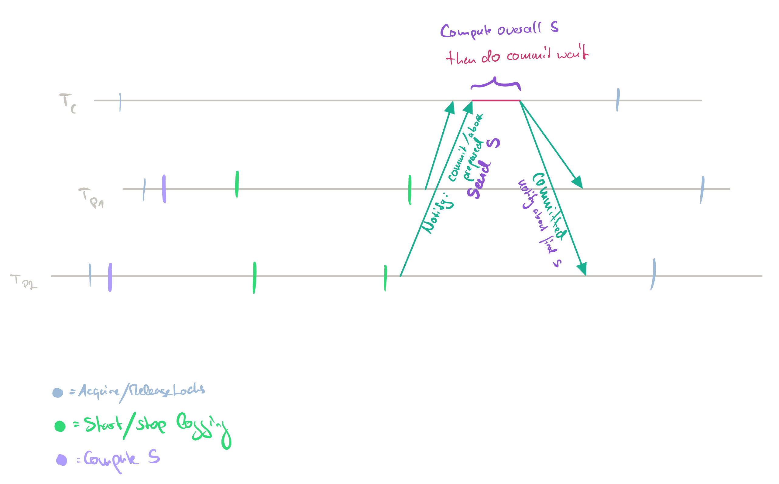
Sharded TX. Each TX takes place on a different shard. T_c leads the TX.
Finally, Spanner’s architecture is shown in the following images:
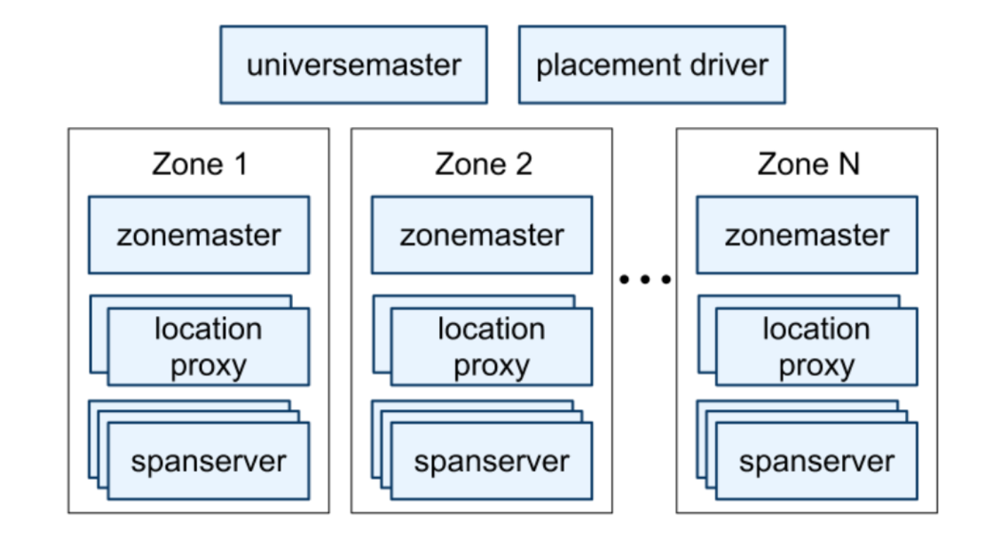
Spanner server organization. Source
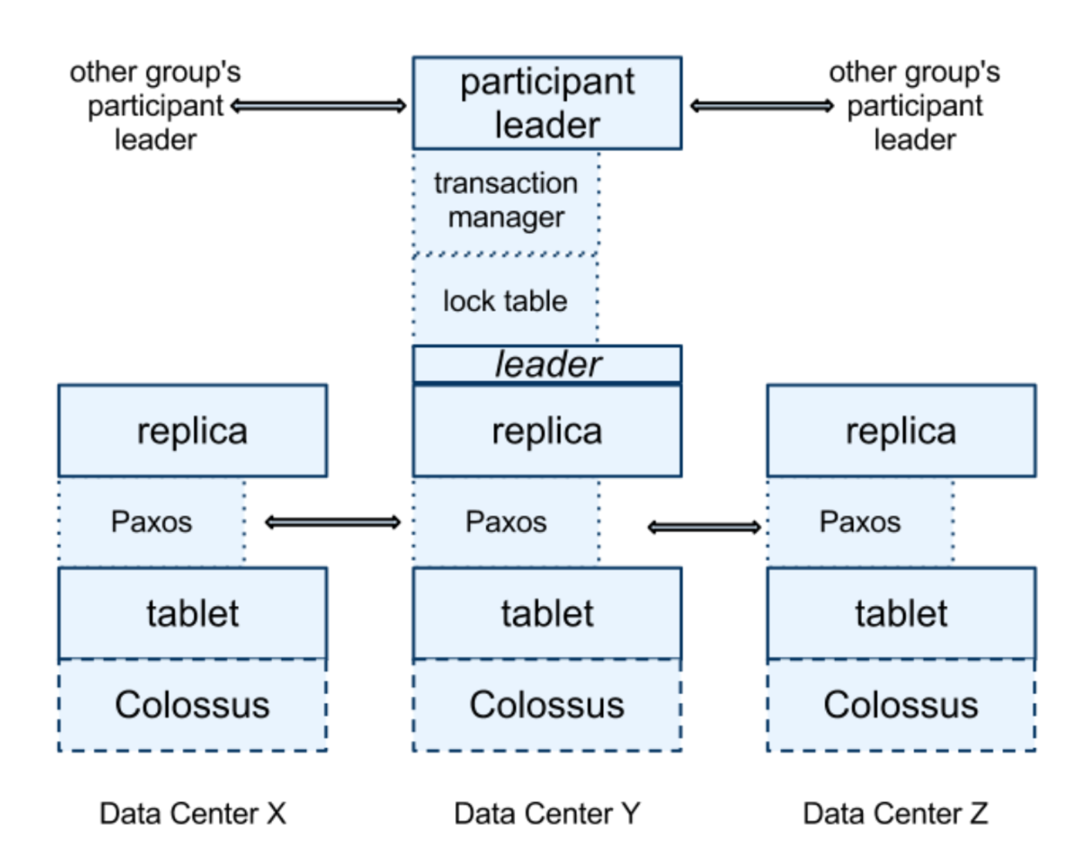
Spanserver software stack. Colussus is similar to GFS. The lock table is used for 2PL. The participant leader(s) run 2PC. Source